
How to use Vlookup in Excel like a pro
Spending too much time trying to find data in a large range of cells?
Well, we have good news! You can use Vlookup.
Vlookup is used to look for a piece of information. Vlookup is short for vertical lookup. It is designed to work with data in a column. To find a specified value it searches for the specific value in one of the columns in the data set and shows you the corresponding values from another column.
In this blog, we are going to look at:
The formula for the Vlookup function
=VLOOKUP(lookup_value, table_array,col_index_num,[range_lookup]) Lookup_value is what you are looking for. It will find the specific values you are searching for in your data set. Table_array is where Excel needs to look for the value you are looking for. Your data needs to be in a table format to use Vlookup. The Vlookup function searches in the most left column of the array. Col_index_num specifies the column you would like to search in. The column is identified by an integer. Range_lookup is the only argument that is not required but a good one to have. It defines what the function should say when it is unable to find the exact match. It is normally set to TRUE or FALSE. When Vlookup finds the exact match it will say TRUE and if an exact match is not found it will return an error, therefore saying FALSE. |
Tips for using Vlookup
- Organise your data: you need to ensure that Vlookup is the appropriate search option for your data. Your data needs to be well organised with what you are looking for on the left-hand side. Vlookup works from left to right so if your data is in the incorrect order Excel will return an error rather than what you are looking for. This is considered to be one of the major drawbacks.
- Indicate what you are looking for: select the cell that contains the information you are looking for.
- Indicate where to look for the data: you need to specify where the data is located, and then tell Excel to search in the leftmost column for the information you are looking for.
- Indicate the column that contains the data: each column in Excel is labelled with a letter of the alphabet, although when we are telling Excel where we would like to search we indicate the column by a number. A corresponds with 1, B with 2, and so on.
- Select which type of match: you can choose either an exact or an approximate match. It is done by choosing either TRUE or FALSE. If you would like an exact match then you select FALSE. If you select TRUE you will get an approximate match.
The Vlookup formula explained
FALSE (Exact match) example:
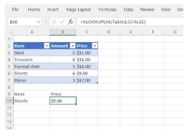
Here we have a list of clothing items that may be in a small retail store. The shopkeeper uses the list to see how much stock they have and quickly sees the price of things using the Vlookup formula. Here we can see the shopkeeper wanted to see the price of shorts. The price is $9.00.
=VLOOKUP(A6;Table1;3;FALSE)
A6 is the lookup_value. We are searching for Shorts, therefore the text string is “Shorts.”
Table1 is the table_array. This table is made up of columns showing the item, the amount, and the price. The Vlookup function will look in the leftmost column (column A) when it is searching for shorts.
3 is the column Vlookup should be looking in. At the top of our columns it says C and that corresponds with the value 3.
False is the range_lookup that requires an exact match. If an exact match is not found the Vlookup function should return an error.
TRUE (An approximate match) example
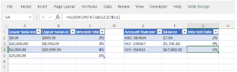
In this example, you can imagine you are working at a bank. You would like to know the interest rates for individual bank accounts. Using the Vlookup function you can determine what interest rate would apply to the amount that is in their bank account. Here we have two tables. The first table shows which rate is applied to the amount of money that is in their bank account. It has a lower balance, and upper balance, and the interest rate that applies. Using the Vlookup function you can easily find the interest rate applicable.
=VLOOKUP(F4;TABLE2;3;TRUE)
F4 is the lookup_value. It is the value you are searching for.
TABLE2 is the table_array you are searching in. In our example, it is table two that contains all the data for the needed interest rates.
3 is the col_index_number. We are looking for the interest rate in column C. C corresponds to the number 3. The value displayed by the Vlookup function should be taken from the 3rd column.
TRUE is the range_lookup. In this example, it is set to TRUE meaning that the Vlookup function will find the value that is the closest match to the value below. Note that if these values are omitted from the Vlookup formula it is automatically set to TRUE.
Common Vlookup errors
#NA! Error:
This error occurs when the Vlookup function cannot find a match to the specific lookup_value. It could also depend on the range_lookup argument:
- If it is set to TRUE the error may occur as the smallest value in the left hand column of the table_array (the data set we are searching for to find our value) is greater than the lookup_value. It could also occur when the values in the left column of our data set are not in ascending order.
- If it is set to FALSE the error may occur as the exact match to what you are looking for has not been found.
#REF! Error:
- If the col_index_num you have specified is greater than the numbers of the columns in the data set you are searching for.
- The Vlookup formula is trying to reference cells that do not exist. It may be due to relative referencing errors when we copy the Vlookup formula to other cells.
#VALUE! Error:
- If the specified col_index_num argument is less than one or is not recognised as a numeric value.
- The indicated range_lookup is not recognised as TRUE or FALSE.
Showing the incorrect values
This often occurs due to human error so there are a few things you can double-check.
- Are the values on the left hand side? The numbers must be to the left in your data set. The Vlookup formula works from left to right. It is best to sort your data and ensure the values are on the left.
- Is the Vlookup function set to TRUE? If left out, the function will return the closest match to the value you have specified. For this to work properly we need to ensure the left column in our data set is in ascending order.
- Is the col_index_num referring to the correct column? Converting the alphabet to numbers may be a bit tricky. Remember the column is counting from the first column of the table you are using. In some cases, it may not be the same as the spreadsheet column number.
- Is the range_lookup set to FALSE? Setting the range_lookup to FALSE requires the formula to find an exact match. Check your data set to ensure there is only one match for the look_up value in the left column. If there is more than one match your Vlookup formula will automatically select the values according to the first match found.
Important things to remember
- If you leave range_lookup out the Vlookup function, it will allow the formula to find a non-exact match, but it will give the exact match if there is one.
- The formula always looks right. It will find the information from the column on the right of the first column of the table.
- If there are any duplicate matches the Vlookup function will only show the first matched value.
- If your data has different cases (eg. capital letters) the Vlookup function is not case sensitive.
- If you already have a Vlookup formula in your worksheet, these formulas may break when inserting a new column. Hard-coded column index values won’t change automatically when columns are inserted or deleted.
- Vlookup allows wildcards. These include the asterisk and question marks.
Want to develop your Excel skills even further? Sign up for our MS Excel Course.