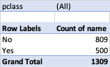
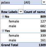
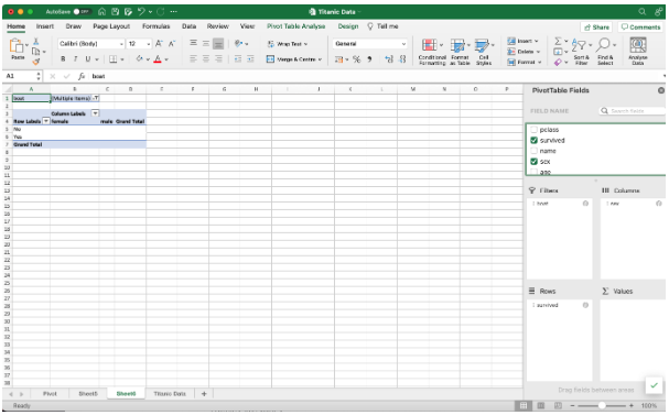
What is the best way to learn Pivot Tables in Excel?

Pivot Table in Excel for beginners

According to Microsoft, a Pivot Table is a powerful tool to calculate, summarise and analyse data. Any person who understands Pivot Tables is likely to agree. It allows you to see comparison patterns and trends as well as quick summaries of key pieces of information.

For those unfamiliar with excel, it’s best to see its power in action.

Pivot Table example in Excel

Let’s say for example you want a comparison of survivors of the Titanic tragedy. Instead of weaving through 1309 lines of items, a Pivot Table can be used to summarise the information.

Data

Pivot Table

Pivot Table Chart

In one quick action, you can get the information you need, displayed in an easy-to-read format.

Pivot Tables also allow for further dissecting and investigation. Let’s say we want to know how many males versus females survived:

Pivot Table

Pivot Table Chart

Or perhaps, did everybody who got into a lifeboat survive?

Pivot Table

Pivot Table Chart

Why we use Pivot Tables in Excel

Pivot Tables provide an interactive way to quickly summarise large amounts of data.

As per our examples above, from the same list of information, key points could be summarised from different perspectives with one or two effortless clicks. By adding Pivot Charts we were also able to visualise the data with no additional effort.

In addition, Pivot Tables can be created from external data sources including:

  • SQL Server tables
  • SQL Server Analysis Services cubes
  • Axure Marketplace
  • Office Data Connection (.odc) files
  • XML Files
  • Access databases
  • Text files
  • Existing Pivot Tables

How to use Pivot Table in excel

Pivot Tables all start with a data list. For the purpose of this article, we’ll continue to use the Titanic data which you can download here if you want to practice along.

In overview, to create a Pivot Table we’ll follow these easy steps:

Step 1: Open the data list

The first step is to open your data list. For the purpose of this article, we’ll use a data list already in excel but as mentioned previously you can import data from a variety of sources, and we invite you to learn more about this in the Upskillist Excel Course.

Step 2: Select the data range

With the data open, select all the rows and columns of which you’d like to view summarised data.

Top tip: To select all columns, click on Cell A1 and simply hold Ctrl, Shift + right arrow. To select all rows, hold Ctrl, Shift + down arrow.

Step 3: Create a Pivot Table

Once selected, click on ‘Insert’ and then select ‘Pivot Table’.

The pop-up window will confirm the table range selected. To proceed simply click ‘OK’

Step 4: Manipulate the Pivot Table display by selecting filters, rows, columns, and values

In the following window, you have the skeleton of your Pivot Table and now simply need to add the data you want to view.

To the right of the page, you will see the ‘PivotTable Fields’. This window allows you to select data that will be displayed in the corresponding field of your Pivot Table.

A Pivot Table is made up of 5 elements, fields, filters, rows, columns and values.

Fields:

The ‘Fields’ window now displays the column headings of your data as a list. Once selected the data from that column will be used to populate the Pivot Table.

These fields will also automatically be selected once pulled into one of the other windows.

Filters:

Filters apply limits to the entire list of data.

Let’s say, for example, we’d like to see the survival rate of those who managed to reach a lifeboat.

We are therefore only interested in the data involving a lifeboat.

To apply a filter, simply:

  1. Drag and drop the appropriate columns, in this case, ‘boat’ to the ‘Filters’ window. You will now see a filter appear on your excel sheet as the Pivot Table starts to populate.
  2. In the Pivot filter, unselect blank entries – in other words, entries where a boat was not allocated. 
  3. The filter display will change from ‘All’ to ‘(Multiple Items)’ as an indication that you are viewing limited data.

Top tip: multiple filters can be applied if needed.

Columns and Rows:

Depending on the data and the preferred display, column titles can be dragged and dropped to the ‘Rows’ window, to be displayed as rows in your Pivot Table or to the ‘Columns’ window to be displayed as columns.

The best thing here is to change the view to see what works best for you.

For the purpose of our scenario, let’s add the ‘Survival’ details to the ‘Rows’ window and ‘Sex’ details to the ‘Columns’ window.

You will now see that B5 will display the number of females who did not survive even after managing to get to a lifeboat, C5 will similarly display the number of males that did not survive and B6 and B7 will display the number of females and males that did survive, respectively.

Now all we need are values, which is where the ‘Values’ window comes in.

Values:

The ‘Values’ window represents the information that will be counted or the sum of values. 

Top tip: Where a column containing text is inserted in the value window, the Pivot will automatically display the number of cells containing text (count).

In the ‘Values’ window, you want to add the column containing the values that should be counted.

For the purpose of our scenario, we’d like to count the number of passengers, and can therefore add ‘name’ to the ‘Values’ window.

And as easy as that, we have a PivotTable, and can now confirm that a total of 9 passengers did not survive even after reaching a lifeboat of which 1 was female and 8 were male.

When to use Pivot Table in excel

Right, we understand that dissecting the Titanic survival rate is hardly something you’ll use in the workplace, but it does provide an interesting way to play around and test the Pivot Table functionality, which we hope you will continue to explore.

In reality, however, here are some practical examples and benefits of making use of Pivot Tables.

Sorting by category

A Pivot Table makes it possible to automatically sort or count values of rows with something in common.

As you noted with our example, females and males were automatically sorted and presented together.

As a more practical example, a list of employees including their departments and job descriptions can effortlessly be arranged to display the number of employees per department or the number of employees with the same job description. 

Calculating totals per category 

Similar to the above function, Pivot Tables can also calculate the sum per category. 

For example, a list of sales of product 1, product 2, and product 3, concluded in a month can be manipulated to reveal the value of sales per product or number of sales per product, and simultaneously provides a valuable comparison between the products.

If you’d like to test this with the Titanic data, add the ‘fare’ column to the ‘Values’ window and see the total ticket costs.

Viewing percentages of a total 

By right-clicking on the cell carrying the total value, it’s possible to select ‘Show Values As > % of Grand Total’. 

This changes the total count or sum value to the % of the Grand Total. 
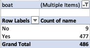
Combining duplicate data 

Pivot Tables summarise per category, thus duplicate values and their corresponding data will automatically be combined when presented in a Pivot Table format.

This is helpful when data is inserted by multiple sources or in multiple instances to purposefully add different data per category.

Adding default values to empty cells 

Right-click on the Pivot Table and click the PivotTableOptions. In the window that appears. Check the ‘Empty Cells As’ box and insert the name of the value you’d like to display instead of a blank cell.

This value will override any blank cell and is helpful when information is still to be confirmed or not relevant to the report. 

Conclusion

Excel can be daunting to any beginner but is indeed a powerful tool with multiple applications. It can streamline and simplify many tasks from business reporting to personal budgets.

To learn more sign up for the Upskillist Excel Course to take you from novice to expert.

To learn more about how Upskillist can help you click the button below :
LinkedIn
Recent Posts