
How to use Hlookup in Excel like a pro
When you are trying to find data in a large range of cells you can use Hlookup. Hlookup is used to look for a piece of information in a large data set.
Hlookup is short for horizontal lookup. It is designed to work with data in rows. To find a specified value it searches for the specific value in one of the rows in the data set and shows you the corresponding values from another row.
The formula for the Hlookup function is:
=HLOOKUP(lookup_value, table_array,row_index_num,[range_lookup])
Lookup_value is what you are looking for. It will find the specific values you are searching for in your data set.
Table_array is where Excel needs to look for the value you are looking for. Your data needs to be in a table format to use Hlookup. The Hlookup function searches in the most left column of the array.
Row_index_num specifies the row you would like to search in. The row is identified by an integer.
Range_lookup is the only argument that is not required but is good to have. It defines what the function should say when it is unable to find the exact match. It is normally set to TRUE or FALSE. When Hlookup finds the exact match, it will say TRUE, and if an exact match is not found it will return an error, therefore saying FALSE.
Using Hlookup
- Organise your data: you need to ensure that Hlookup is the appropriate search option for your data. Your data needs to be well organised with what you are looking for in the first row of the table. Hlookup works from top to bottom so if your data is in the incorrect order Excel will return an error rather than what you are looking for. This is considered to be one of the major drawbacks.
- Indicate what you are looking for: select the cell that contains the information you are looking for.
- Indicate where to look for the data: you need to specify where the data is located, and then tell Excel to search in the leftmost column for the information we are looking for.
- Indicate the row that contains the data: each row in Excel is labelled with a number.
- Select which type of match: you can choose either an exact or an approximate match. It is done by choosing either TRUE or FALSE. If you would like an exact match then you select FALSE. If you select TRUE you will get an approximate match.
FALSE (Exact match) example:
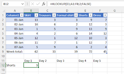
Here we have a list of clothing items that may be in a small retail store. The shopkeeper uses the list to see how much stock is sold. He uses this information to see how many new items he needs to order to replenish his stock at the end of the month. Instead of finding the corresponding values manually, he decides to use the Hlookup formula. We can see on the first day of the week 9 pairs of shorts were sold.
Formula explained:
=HLOOKUP(E1;A1:F8;2;FALSE)
E1 is the lookup_value. We are searching for Shorts, therefore the text string is “Shorts.”
A1:F8 is the table_array. This table is made up of columns showing the item, the day of the week, and the number of items sold. The Hlookup function will look in the top row (E1) when it is searching for shorts.
2 is the row Hlookup should be looking in.
False is the range_lookup that requires an exact match. If an exact match is not found the Hlookup function should return an error.
TRUE (An approximate match) example
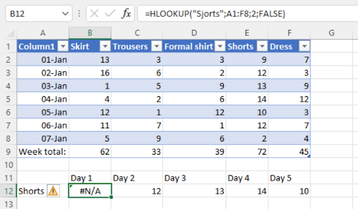
While the shopkeeper is typing the word Shorts his finger slips and he puts the letter j instead of the h. It results in him looking for the word “Sjorts” instead of Shorts. As Excel does not have an exact match for the word it results in a #NA! error.
Formula explained:
=HLOOKUP(F4; TABLE2;3; TRUE)
Sjorts is the lookup_value. We are searching for Shorts, therefore the text string is “Shorts.” But as we see in this example the shopkeeper has made a mistake.
A1:F8 is the table_array. This table is made up of columns showing the item, the day of the week, and the number of items sold. The Hlookup function will look in the top row (E1) when it is searching for shorts.
2 is the row Hlookup should be looking in.
True is the range_lookup that requires an approximate match. If an exact match is not found the Hlookup function should return an error.
Hlookup errors
#NA! error:
This error occurs when the Hlookup function cannot find a match to the specific lookup_value.
- If it is set to FALSE the error may occur as the exact match to what you are looking for has not been found.
- If there is a combination of real dates or times and string (text) date or times.
#REF! error:
- If the row number entered into the formula is bigger than the number of rows in the table.
- It may occur if you deleted some of the rows in the table and the formula is not updated.
#VALUE! Error:
- If the row number entered is smaller than 1 an error will occur.
- It may occur when a cell is empty or has a zero and you try to refer to it.
Important things to remember when using Hlookup
- If you leave range_lookup out the Hlookup function will allow the formula to find a non-exact match, but it will give the exact match if there is one.
- The formula always looks right. It will find the information in the top row of the table.
- If there are any duplicate matches the Hlookup function will only show the first matched value.
- If your data has different cases (eg. capital letters) the Hlookup function is not case sensitive.
- Hlookup allows wildcards. These include the asterisk and question marks.
Learn how to use Excel like a pro.